Numerical Simulation of Constant Cadence Approximation

A big issue with power accuracy is to not only get the force versus time accurate but also to get an accurate cadence versus time. Power is the instantaneous product of propulsive force times pedal velocity, pedal velocity being proportional to cadence multiplied by crank length, and therefore errors in cadence translate directly to errors in power.

It is typical in the power meter business that cadence is approximated as constant over a full or perhaps half pedal stroke. Indeed, Garmin has announced they are using this approximation on the Vector. This is of course technically incorrect: cadence varies over a given pedal stroke just as it varies from one pedal stroke to the next. Ideally cadence would be sampled at a sufficient rate to get multiple points within a half-pedal-stroke, so the variation in pedal speed between the strong and weak portions of the pedal stroke would be captured.

I have previously looked at this issue and I concluded the power error would be proportional to the correlation coefficient between pedal force and pedal speed. If the resistance was very strong, which is the limit of a zero-inertia condition, then the two would be perfectly correlated. On the other hand, if inertia is dominant, the rate of change of the pedal speed rather than the pedal speed itself will be proportional to the force, and this will result in a low correlation coefficient. So the question is which of these two conditions applies in real-life cycling.

For completeness, I'll put the relationship between correlation and error here:

The constant cadence approximation makes the following assumption for each pedal stroke:

<τ × ω> = <τ> × <ω>

where ω is the angular velocity of the pedals, τ is the propulsive torque, and brackets signify a time-average.

The error from this approximation is obviously:

<τ> × <ω> − <τ × ω>

which is fairly trivially shown to equal:

− <(τ - <τ>) × (ω − <ω>)>

which is proportional to the correlation coefficient between torque and angular frequency, where a positive correlation results in an underestimation of power.

Metrigear published instantaneous cadence data measured with their Speedplay Vector prototypes. These data showed cadence varied substantially around the pedal stroke. Indeed those data suggested the correlation was substantial, and therefore the power error associated with a constant cadence approximation would be significant relative to a 2% power accuracy target. However, the accuracy of these cadence variations was uncertain. Even 1% accuracy on cadence is insufficient if the goal is to gain accuracy on the variation of cadence, where the variation is on order 1% of the mean. So determining the correlation between cadence and force from those data would be risky. Additionally, the data applied to a particular riding condition, for example an indoor trainer, which is not generally representative. I wanted to be able to analyze a variety of conditions.

So I recently decided to try something different. I took the Metrigear power-versus-time data for the left and right foot. I then took used their cadence data to convert time to a pedal angle. This produced a nice periodic, regular pedal stroke for each foot as long as I increased these cadence numbers by 1.5%. I therefore assumed that the pedal power versus angle was fixed, while pedal speed could be determined from physics. Given a rider mass, a gear development, a road grade, a coefficient of rolling resistance, a wind resistance coefficient, a wind speed, and an inertial mass ratio I could calculate the cadence as a function of time from this power as a function of angle. This is a self-consistent calculation (to calculate watts I need angle, to determine angle I need speed, to know speed I need watts). So I iterated the solution for each time-step until it was self-consistent. With this approach I could test the constant cadence approximation for different road grades, different cadences, during periods of acceleration versus steady-state, and even compare one-legged versus two-legged pedaling.

To pad out the data from Metrigear, the plot showing only three complete pedal strokes, I replicated the data to create a repeating series of three pedal strokes. Each of the repeating sequences would differ slightly due to inertia.

For inertia, I assumed 102% of total mass. It's not exactly equal to total mass due to the rotating mass effect of the wheels and tires. I made various "reasonable" assumptions about rolling resistance, wind resistance, transmission losses, rider and bike mass, etc.

With this approach, I can test the error associated with the constant cadence approximation for different pedal strokes under different conditions. For example, here was the result for pedaling on flat ground with no wind, starting from 40 rpm but ramping up toward 90 rpm:

nrot dt       avgrpm  avgwatts avgtorque avgwattsCC err       ferr
0    1.35538  44.1263 422.339  9.40279   414.91     -7.42958  -0.0175915
1    1.17845  50.9276 388      7.55999   385.012    -2.98736  -0.00769938
2    1.07454  55.8079 378.433  6.74782   376.582    -1.8515   -0.00489255
3    0.997814 59.9389 424.597  7.06713   423.596    -1.00106  -0.00235767
4    0.950991 63.1089 389.941  6.1571    388.568    -1.37369  -0.00352281
5    0.912108 65.7464 379.463  5.75707   378.506    -0.956906 -0.00252173
6    0.876475 68.2356 425.084  6.22075   424.477    -0.607937 -0.00143016
7    0.854664 70.2218 390.54   5.54978   389.715    -0.82464  -0.00211154
8    0.833606 71.9376 379.85   5.27197   379.253    -0.597296 -0.00157245
9    0.812025 73.6507 425.294  5.76878   424.875    -0.419305 -0.000985918
10   0.799999 75.0202 390.827  5.20225   390.274    -0.553386 -0.00141594
11   0.786445 76.2202 379.958  4.97967   379.552    -0.406289 -0.0010693

The columns are: rotation number, seconds for that rotation, average rpm during that pedal stroke, average watts for the pedal stroke, average torque (nonstandard units: power divided by rpm), and the average watts calculated per the constant cadence approximation. Then I show the error in watts, and the fractional error, associated with the constant cadence approximation.

During the first pedal-stroke, the error is 1.8%. This isn't good, but the bike is strongly accelerating here. As the speed becomes more constant, the error of the constant cadence approximation is reduced. It drops to a small fraction of a percent in the latter pedal stroke.

The first question is what happens when the pedal stroke is less uniform, for example pedaling right leg only? For this, I took the right leg data only, truncating negative powers to zero (to avoid the risk of the cadence dropping to zero). I automatically adjust the rider's gear to yield the same initial and target cadence. Here's that result:

nrot dt       avgrpm  avgwatts avgtorque avgwattsCC err       ferr
0    1.41507  42.2648 224.381  5.0463    213.281    -11.1     -0.0494694
1    1.23773  48.4886 236.113  4.76911   231.247    -4.86513  -0.0206051
2    1.12117  53.4869 223.193  4.12155   220.449    -2.74437  -0.0122959
3    1.04627  57.1625 228.249  3.95441   226.044    -2.20493  -0.00966019
4    0.997117 60.1895 238.918  3.9306    236.581    -2.33734  -0.009783
5    0.951472 63.0263 224.556  3.53946   223.079    -1.47637  -0.00657462
6    0.916343 65.2666 229.201  3.4919    227.905    -1.29648  -0.00565653
7    0.892921 67.2132 239.836  3.54645   238.369    -1.46727  -0.00611783
8    0.867219 69.1493 225.095  3.24135   224.137    -0.957759 -0.00425491
9    0.845919 70.6995 229.626  3.23548   228.747    -0.87909  -0.00382836
10   0.832684 72.0755 240.286  3.31948   239.253    -1.03282  -0.00429831
11   0.815539 73.5022 225.203  3.05467   224.525    -0.677269 -0.00300738

It can be seen during the first three pedal strokes, starting from 40 rpm, the error exceeds 1%, as large as 5%. However, the error during the later pedal strokes is on order 0.5%. This is nontrivial, but not terribly bad, despite the abnormally rough pedal stroke.

Then I considered the effect of road grade. I'll assume a lower target cadence, 50 rpm, with a grade of 20%. This is extreme hillclimbing. I'll start at 50 rpm:

nrot dt    avgrpm avgwatts avgtorque avgwattsCC err     ferr
0    1.207 49.54  422.3    8.389     415.6      -6.709  -0.01589
1    1.218 49.27  389.4    7.882     388.4      -1.009  -0.00259
2    1.225 48.95  378.8    7.725     378.2      -0.5963 -0.001574
3    1.171 51.07  423.1    8.249     421.3      -1.784  -0.004218
4    1.205 49.82  389.8    7.81      389.1      -0.6728 -0.001726
5    1.22  49.14  378.9    7.7       378.4      -0.4862 -0.001283
6    1.17  51.13  423.1    8.24      421.3      -1.761  -0.004163
7    1.204 49.85  389.8    7.807     389.1      -0.6588 -0.00169
8    1.22  49.15  378.9    7.699     378.4      -0.4813 -0.00127
9    1.17  51.14  423.1    8.239     421.3      -1.76   -0.004161
10   1.204 49.85  389.8    7.807     389.1      -0.6583 -0.001689
11   1.22  49.15  378.8    7.698     378.4      -0.4779 -0.001261

Next I'll try headwind, assuming riding at 70 rpm target into a 5 mps headwind:

0  0.8549 69.96 425.6 6.018 421   -4.587    -0.01078
1  0.8583 69.92 391.3 5.596 391.3 -0.04421  -0.000113
2  0.8585 69.85 380.4 5.446 380.4 -0.01177  -3.094e-05
3  0.854  70.04 425.6 6.075 425.4 -0.1448   -0.0003401
4  0.8575 69.99 391.3 5.591 391.3 -0.04024  -0.0001028
5  0.8577 69.91 380.4 5.442 380.4 -0.00877  -2.305e-05
6  0.8533 70.09 425.6 6.07  425.4 -0.1429   -0.0003358
7  0.8569 70.03 391.3 5.587 391.3 -0.03759  -9.606e-05
8  0.8573 69.95 380.5 5.439 380.4 -0.006768 -1.779e-05
9  0.8529 70.12 425.6 6.067 425.4 -0.1417   -0.0003329
10 0.8566 70.06 391.4 5.585 391.3 -0.03583  -9.154e-05
11 0.8566 69.98 380.4 5.435 380.4 -0.005154 -1.355e-05

So far, only during rapid acceleration is the error worth worrying too much about. On the other hand, if I suspend inertia, things are very different. Here's what I get if I assume speed (and rpm) responds instantly to power fluctuations:

nrot dt     avgrpm avgwatts avgtorque avgwattsCC err    ferr
0    0.9424 63.47  362.4    5.037     319.7      -42.75 -0.118
1    0.997  60.2   324      4.69      282.3      -41.64 -0.1285
2    1.039  57.73  302.5    4.432     255.9      -46.66 -0.1542
3    0.9415 63.52  362.2    5.081     322.8      -39.43 -0.1089
4    0.997  60.2   324      4.69      282.3      -41.64 -0.1285
5    1.039  57.73  302.5    4.432     255.9      -46.66 -0.1542
6    0.9415 63.52  362.2    5.081     322.8      -39.43 -0.1089
7    0.997  60.2   324      4.69      282.3      -41.64 -0.1285
8    1.039  57.73  302.5    4.432     255.9      -46.66 -0.1542
9    0.9415 63.52  362.2    5.081     322.8      -39.43 -0.1089
10   0.997  60.2   324      4.69      282.3      -41.64 -0.1285
11   1.038  57.73  302.4    4.431     255.8      -46.65 -0.1543

The error is enormous, but this condition would be approximated only when riding a trainer with a low-mass flywheel.

These results can be understood by looking at how power and rpm are related. I plot watts on the y-axis, rpm on the x-axis for the final three of my 12-pedal-stroke simulation (recall there's only three unique pedal strokes, which I replicate). Here's 3 cases.

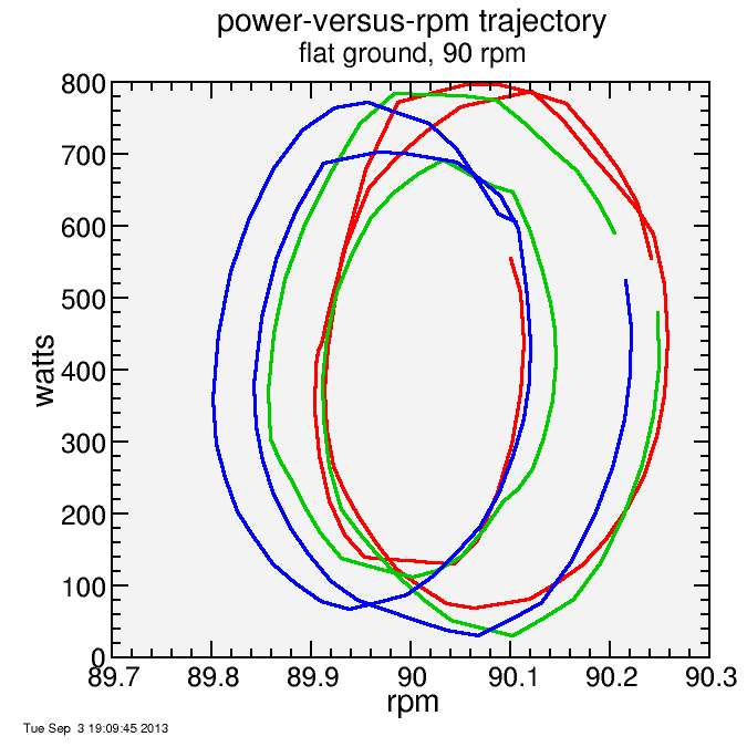
First, riding at 90 rpm on flat ground:

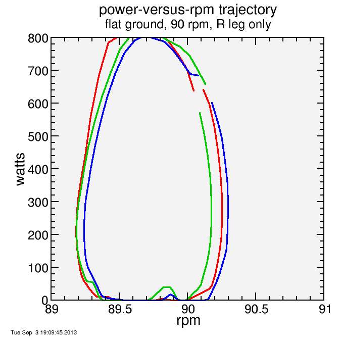
Then, the same condition except riding right-foot-only:

Then at 40 rpm on a 20% grade:

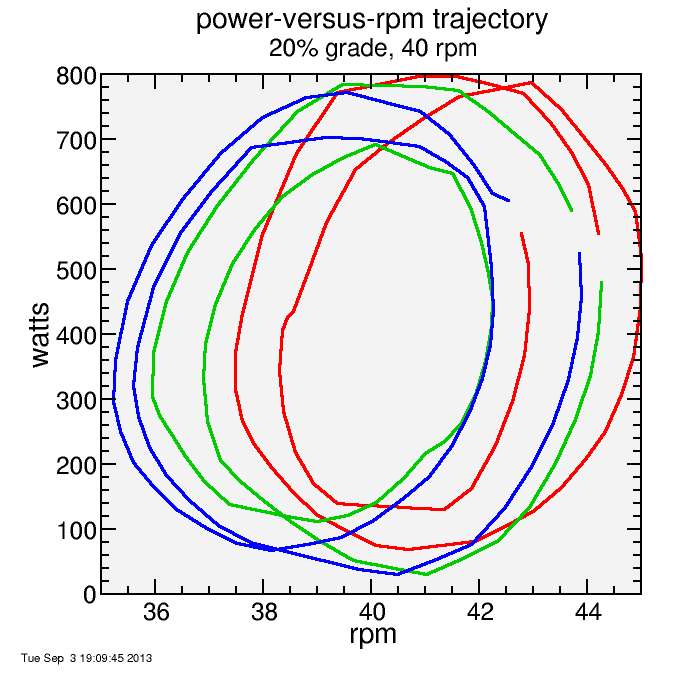
In each of these conditions inertia is sufficient that rpm and watts over a given pedal stroke are poorly coorelated, so errors in cadence associated with assuming cadence is constant over a pedal stroke generally cancel: for the same power, there are cadence values relatively equally distributed above and below the average, so assuming the average is a decent approximation.

However, when I assume inertia is zero I get the following:

Here power and cadence are perfectly correlated. Above-average powers tend to have higher-than average cadence, while below-average powers tend to have below-average cadence. The constant cadence approximation is a poor one.

So the result of all of this is I think, for round chainrings, that over a given pedal stroke inertia has a strong influence in real-life riding conditions and the constant cadence approximation isn't too terrible an error. On a trainer, inertia will be relatively small without a heavy fly-wheel (or computer control) and the constant cadence approximation may not do as well.

Eccentric chainrings, however, are another matter. Their whole purpose is to correlate power and cadence. With them, the errors will be larger than for round chainrings.

Garmin is well aware of this issue and have stated that using the constant cadence approximation with round chainrings doesn't violate their claimed power accuracy. Indeed, except for unusual circumstances, like rapid accelerations from low cadence, and exceptionally low inertia conditions, it appears that statement is justified.